Adversarial Attack
- For a trained network, we need to ask whether it is robust enough to handle malicious inputs and prevent the model from being fooled.
- We hope the network not only has high accuracy, but also has the ability to resist deceptive malicious inputs.
- Given an original benign image, one can add tiny perturbations to each pixel to generate an attacked image, causing the model to make an incorrect classification.
- Attacks can be divided into targeted attacks and non-targeted attacks. The difference is whether the attacker predefines the wrong prediction that the model should produce.
Attack Methods
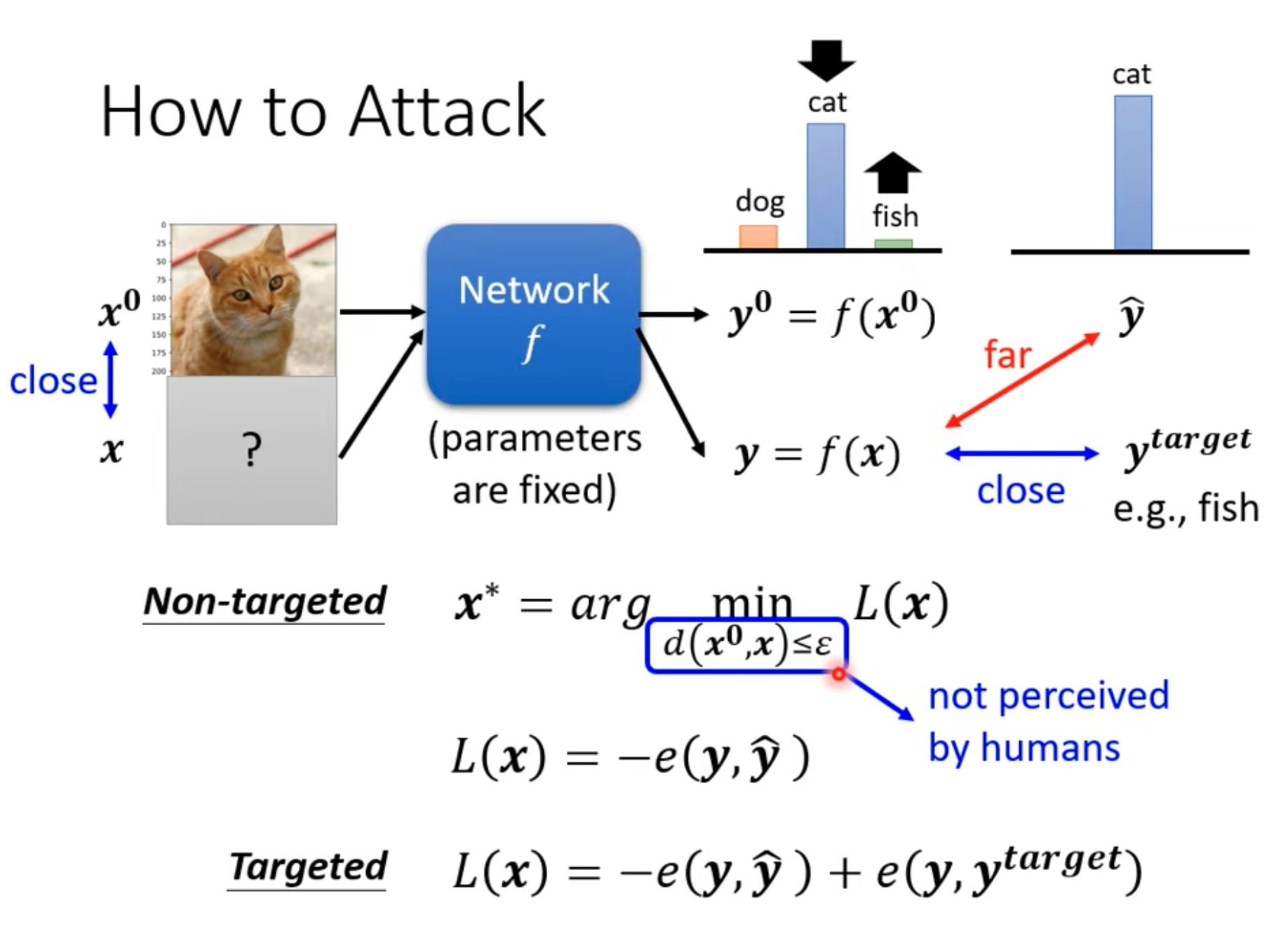
For the model being deceived, since the attack is performed after model deployment, we can treat the model parameters as fixed.
For the original input image $x^0$, the output is $y^0$. For the attacked image $x$, the output is $y$. If the true label is $\hat{y}$, we hope the output $y$ of the attacked image is as far away from $\hat{y}$ as possible. Such a loss function can be defined as the negative cross-entropy. On the other hand, we also want the attacked image to be as similar as possible to the original image. Therefore, we need $d(x^0,x)\le \epsilon$, meaning the image distance should be below a threshold. This distance can be the maximum difference, mean squared difference, or other metrics.
- L2 norm: the sum of squared differences.
- L-infinity: the maximum absolute difference.
- Adjusting every pixel in an image slightly and adjusting only one pixel more strongly may produce the same L2 norm, but the L-infinity distance can be very different.
- From human visual perception, small changes spread across many pixels are harder to notice.
For targeted attacks, we hope the attacked image is far from the true label and close to the target label.
With model parameters fixed, generating an attacked image means optimizing the input $x$ according to the loss function. This is similar to ordinary model training, except that the optimized variable is the input image rather than the model parameters.
During model training:
$$ w^*,b^* = \operatorname*{arg\,min}_{w,b} L(y,\hat{y}) $$When generating an attacked image:
$$ x^* = \operatorname*{arg\,min}_{x} L(x) $$Use gradient descent to obtain $x$:
Initialize the input image as the real image $x^0$.
For each step $t$:
$$ x^t \leftarrow x^{t-1}+\eta \frac{\partial L(x)}{\partial x} $$If $d(x^0,x^t) > \epsilon$, then project or fix $x^t$ back into the allowed perturbation range.
In the procedure above, we use gradient descent to solve for the attacked image. Computing the gradient requires knowing the model parameters, because
$$ g=\frac{\partial L(x)}{\partial x},\quad L(x)=-e(y,\hat{y}),\quad \hat{y}=f_{\theta}(x) $$Here, $\theta$ denotes the model parameters that must be known. This type of attack is called a white-box attack because it requires access to the model parameters. The corresponding setting is the black-box attack.
Black-Box Attack
- Suppose we do not know the parameters of a model, but we know the dataset used to train it. We can use that dataset to train our own network, whose architecture may be different from the target network. Such a network is called a proxy network. Then we can use a white-box method on the proxy network to compute adversarial images, which may also attack the original model.
- If the training set of the original model is unknown, we can feed many images into the model, collect their output labels, and use these image-label pairs to train our proxy network. This can also produce an effective attack.
- Black-box attacks are usually used for non-targeted attacks.
- Attacks are relatively easy to implement:
- Both black-box and white-box attacks can have high success rates.
- A single-pixel change can be enough to complete an attack.
- One perturbation pattern can attack images from multiple categories.
- Attacks can be realized in the physical world, such as wearing specially designed glasses for face recognition or modifying traffic signs.
- Model backdoor: during model training, specific images are added, and their labels may still appear subjectively correct. After the model is trained on this dataset, it may classify an image incorrectly when a certain trigger appears, even if that image is not necessarily the exact image from the training set.
Defense Methods
Passive defenses:
- Add a filter before the image enters the model. This filter may be a very simple preprocessing operation.
- For example, smoothing or blurring can greatly reduce attacks, because adversarial signals in attacked images are highly specific. Once the image is blurred, the attack signal is affected.
- Compress and then decompress the image.
- Other similar preprocessing operations.
- Filters can also be broken. A filter can be regarded as a hidden layer of the model. If the attacker knows the exact filtering method, the same filter can be included when generating the attacked image, producing a corresponding adversarial example.
- A related defense is to use randomized filters.
Active defenses:
- Train a model that is difficult to attack from the beginning, namely adversarial training, so that the model becomes more robust.
- The main idea is: for a training set $(X,y)$, first train the model, then use a white-box attack to obtain attacked images $X'$. Assign correct labels to the attacked images to obtain $(X',y)$, then merge the two datasets into $(X+X',y)$ and retrain the model. This process can be repeated multiple times.
- This idea can also be viewed as a form of data augmentation.
- The computation is very expensive.