Generator and Generative Models
Basic Structure of Generative Models
- Compared with a traditional discriminative model that takes input $x$ and outputs $y$, a generative model also takes a randomly generated $z$ as input. This $z$ is sampled from some distribution, and the network generates $y$ based on both $x$ and $z$.
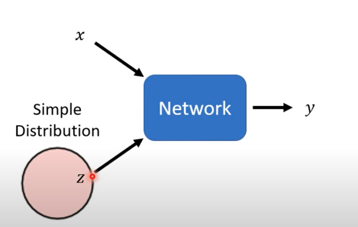
- Every time $x$ is given as input, a new $z$ is generated. The distribution of $z$ must be simple enough, meaning that we need to know its expression. For example, $z$ may follow a Gaussian distribution or a uniform distribution.
- In this way, the same $x$ can produce different outputs $y$, and $y$ also needs to follow some distribution.
Why Generative Models Are Needed
In video prediction, the training set consists of frames extracted from videos, and the model outputs the next frame.
Suppose the video comes from a Pokemon-style game, where a moving object may turn either left or right. In this training data, both left turns and right turns are correct cases for a discriminative model. To maximize accuracy, the model may average the two possibilities, causing the trained model to fail to understand left and right turns correctly.
In other words, the discriminative model is confused by the fact that both left and right turns are correct. It does not know how to choose and ends up trying to please both sides.
For a generative model, the output can be assisted by the sampled probability variable $z$. With some probability, the model predicts a right turn; with some probability, it predicts a left turn. The output is no longer fixed, but becomes a distribution.
In certain scenarios, the same input may have multiple correct outputs. The model needs to decide among these possibilities by itself, so a random variable $z$ is needed to provide a kind of “creativity”.
Image generation requires “creativity”; question-answering chatbots also require “creativity”.
Generative Adversarial Network (GAN)
GAN Example
Unconditional generation, such as generating anime faces:
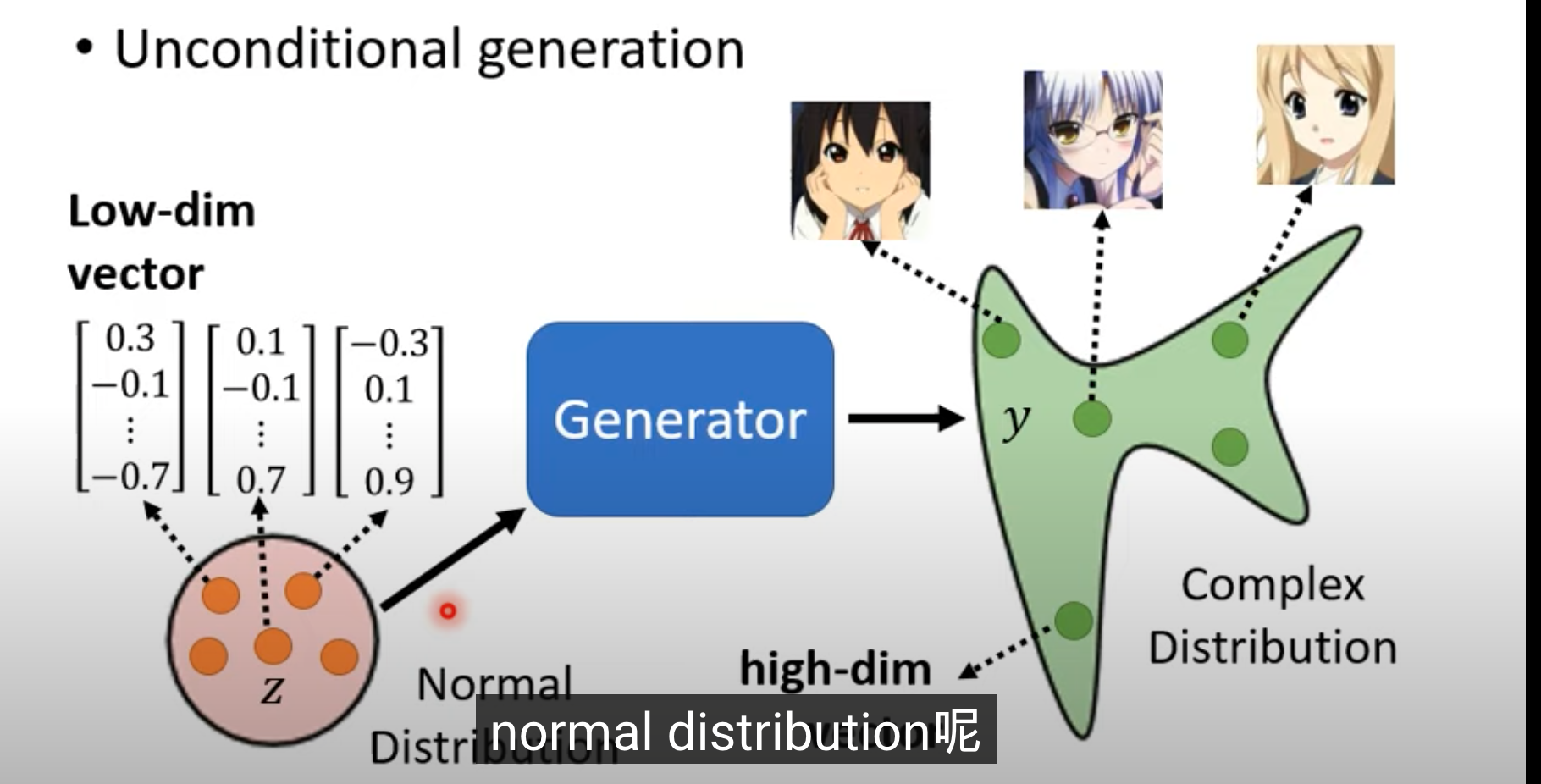
- For now, ignore $x$. The only input is a normally distributed $z$, which is a simple vector. The model generates different images according to different $z$ values. If the image is a $64 \times 64$ color image, the output is a vector of size $64\times64\times3$.
- Besides the generator, we also need a discriminator, which is another neural network. It can use CNN, Transformer, or other architectures. Its input is an image, and its output is a scalar. For a given input image, the larger the scalar is, the more the image matches what we want.
The Idea of GAN
The idea is similar to biological evolution and survival of the fittest. Birds eat colorful butterflies, so the butterflies evolve into brown butterflies. Birds then start to recognize patterns and eat brown butterflies too. The butterflies evolve into dead-leaf butterflies, and birds then learn to distinguish dead-leaf butterflies from real dead leaves.
Here, the evolution of butterflies plays the role of the generator, while the bird plays the role of the discriminator.
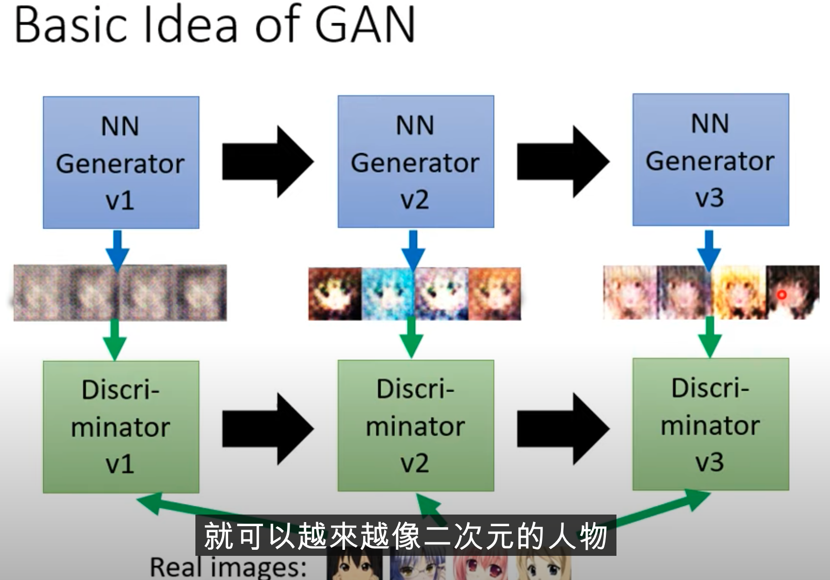
First, the generator randomly produces cases. The discriminator compares them with real images and judges whether a generated image is real based on whether it has eyes. The generator then learns to randomly generate images with eyes. Next, the discriminator judges realism based on whether the image has a mouth and hair. This cycle continues as an evolutionary process.
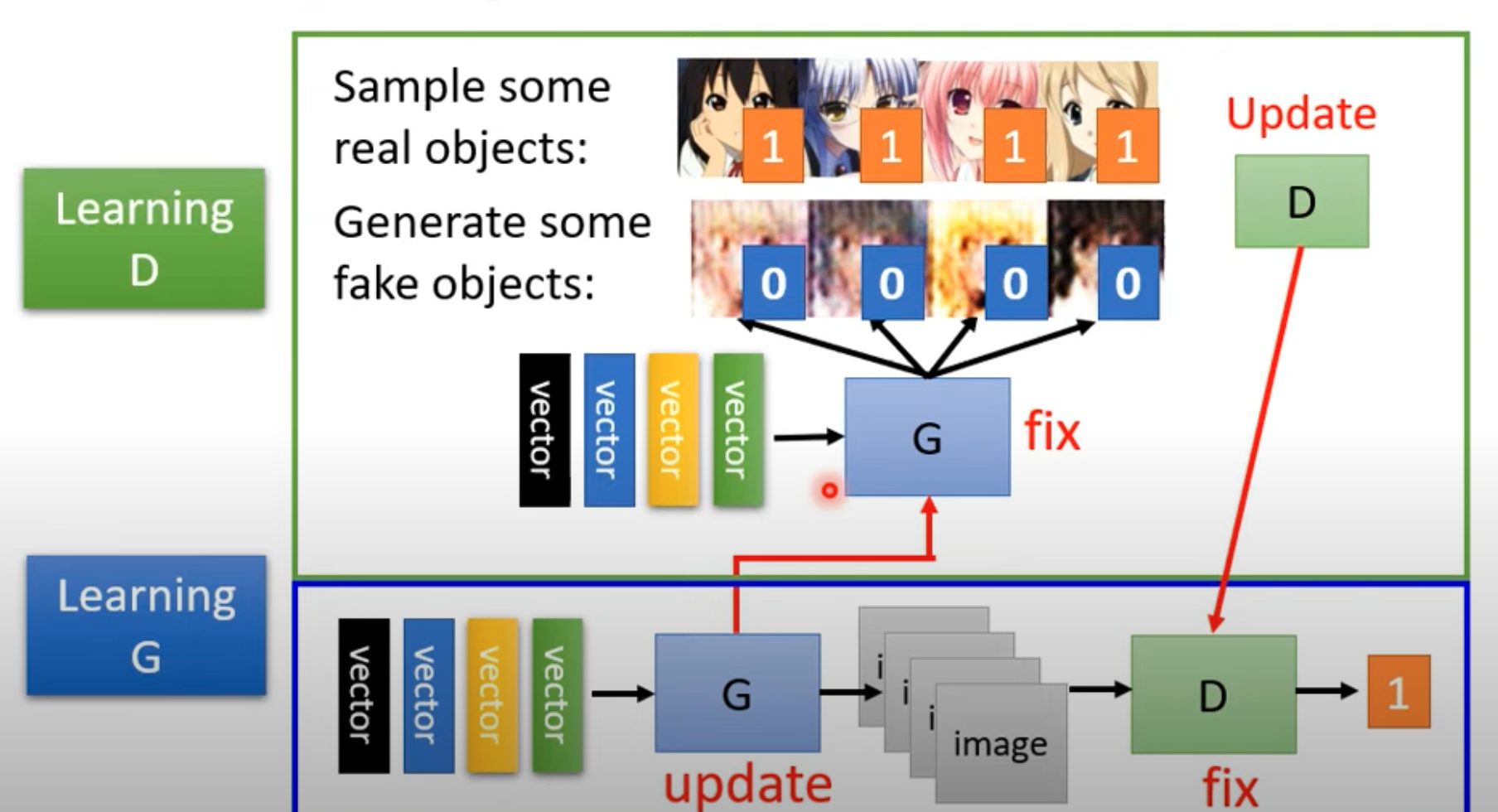
Adversarial Algorithm
Initialize parameters and create the generator and discriminator.
For each training iteration, first train the discriminator:
- Fix the generator and update the discriminator. The generator takes randomly distributed $z$ as input and outputs images according to the random parameters.
- Train the discriminator using real images and generated images so that it can distinguish the two. A concrete method is to label all real images as 1 and all generated images as 0. In this way, the discriminator’s work can be viewed as either a regression problem or a binary classification problem.
Then train the generator:
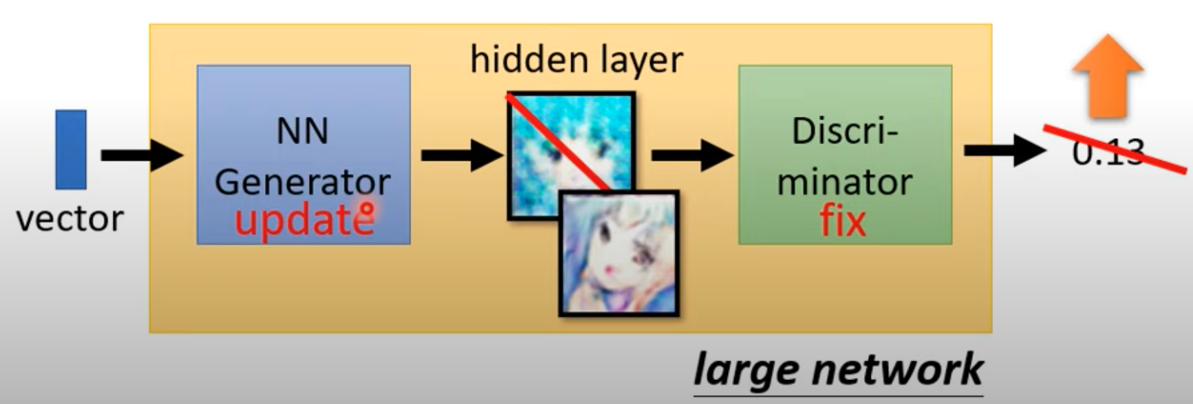
- Fix the discriminator parameters and update the generator parameters. The goal is to make images generated from random $z$ “fool” the discriminator.
- Fooling the discriminator can be understood as making the generated image receive as large a discriminator score as possible.
- Specifically, we can connect the generator and discriminator into one “large network”, where the generated image is treated as a hidden layer of the larger network. The input of this large network is random $z$, and the output is the discriminator’s score.
- We then train this large network and update the parameters of the first half, namely the generator, so that the final output is as large as possible. The loss function needs special design.
Repeat this process, alternately training the generator and discriminator.
Theoretical Analysis of GAN
Training Objective of GAN
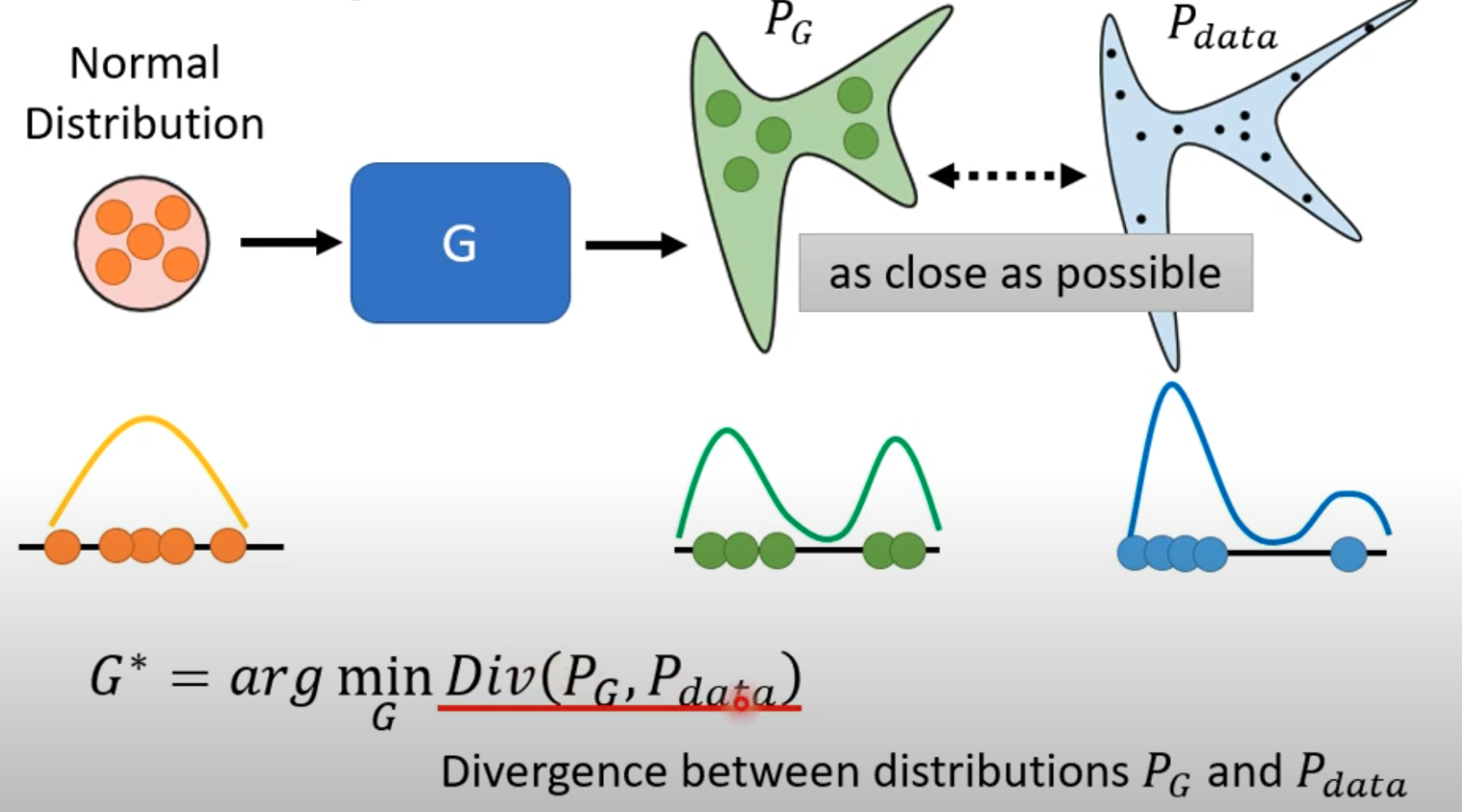
A vector $z$ sampled from a random distribution is fed into the generator, which produces a generated distribution $P_g$. We want $P_g$ to be as close as possible to the real data distribution $P_{data}$.
Divergence refers to the distance between two data distributions, such as KL divergence, JS divergence, and many other distance measures. A key problem is how to compute this divergence from the two kinds of data. Since $P_g$ and $P_{data}$ are two large datasets, direct computation is difficult. The training process can be understood as learning this divergence.
GAN handles this problem by randomly sampling from $P_g$ and $P_{data}$. Sampling from $P_{data}$ means sampling from the real dataset. Sampling from $P_g$ means sampling a random vector $z$ from a known distribution and generating a sample through the generator. In this sense, the generator can be viewed as the dataset of $P_g$.
GAN relies on the discriminator to estimate a way of computing the divergence using samples drawn from $P_g$ and $P_{data}$.
- The discriminator’s task is to distinguish real images from generated images.
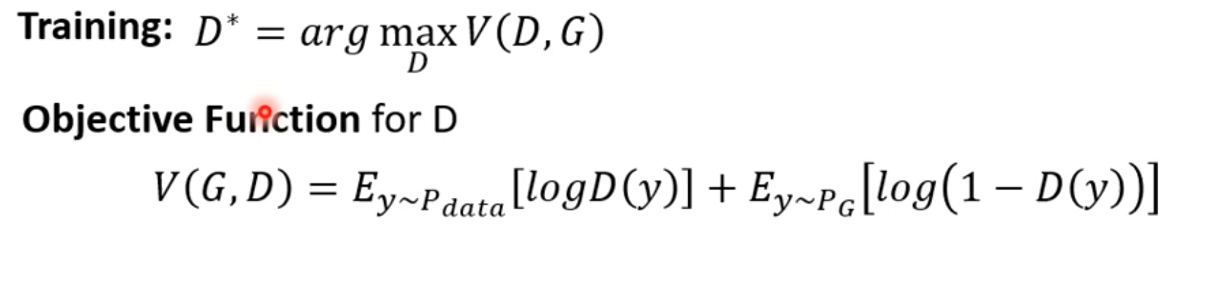
- This is like training a binary classifier. We hope the trained classifier makes $V(D,G)$ as large as possible.
- Here, $V(D,G)$ can be the negative cross-entropy. Since the objective in a binary classification problem is usually to minimize cross-entropy, using negative cross-entropy means we want to maximize it.
- The key point is: no matter how the discriminator is trained, our objective is to maximize the discriminator’s objective function.
- The most important and somewhat magical point is that when the classifier is treated as a classification task and we compute $\max_D V(D,G)$, the derived value is related to the JS divergence. In other words, when directly computing the divergence between the generated distribution $P_g$ and $P_{data}$ is difficult, optimizing the discriminator objective to its maximum provides an evaluation of the current divergence.
- For the full derivation, see Goodfellow’s original GAN paper. Intuitively, the more similar generated images and real images are, meaning the more similar $P_g$ and $P_{data}$ are, the harder it is for the discriminator to distinguish them. The corresponding $\max_D V(D,G)$ becomes smaller, and the corresponding divergence also becomes smaller.
To summarize, the generator’s original training objective is
$$ G^*=\operatorname*{arg\,min}_{G}\operatorname{Div}(P_g,P_{data}) $$Given $P_g$ and $P_{data}$, $\operatorname{Div}(P_g,P_{data})$ cannot be computed directly. Therefore, we use an indirect method: let the discriminator distinguish $P_g$ from $P_{data}$. The discriminator’s training objective is
$$ D^*=\operatorname*{arg\,max}_{D} V(D,G) $$Here, $\max_D V(D,G)$ is positively related to $\operatorname{Div}(P_g,P_{data})$. The harder it is for discriminator $D$ to distinguish $P_g$ and $P_{data}$, the smaller $\max_D V(D,G)$ is, indicating that $P_g$ and $P_{data}$ are more similar and their divergence is smaller. Therefore, we can use $\max_D V(D,G)$ to replace $\operatorname{Div}(P_g,P_{data})$, and the generator’s training objective becomes
$$ G^*=\operatorname*{arg\,min}_{G}\max_D V(G,D) $$
GAN Training Tricks
GAN is famous for being difficult to train.
Take JS divergence and a binary discriminator as an example. In most cases, $P_g$ and $P_{data}$ are just the generated image dataset and the real image dataset. The problem is:
- These images often have little overlap. $P_{data}$ and $P_g$ lie on low-dimensional manifolds in a high-dimensional space. For example, a random image is a randomly sampled point in a $64\times64\times3$ dimensional space, and the probability that it forms a meaningful face image is extremely small. The same applies to $P_{data}$. Therefore, it is difficult for $P_{data}$ and $P_g$ to have matching cases.
- We never know the true distributions of $P_g$ and $P_{data}$. Even if $P_g$ and $P_{data}$ overlap substantially, the sampled cases may not overlap.
Therefore, for JS divergence, as long as two cases do not overlap, the JS value is $\log 2$. No matter how close or far the samples from $P_g$ and $P_{data}$ are, as long as they do not exactly overlap, the JS distance will be large.
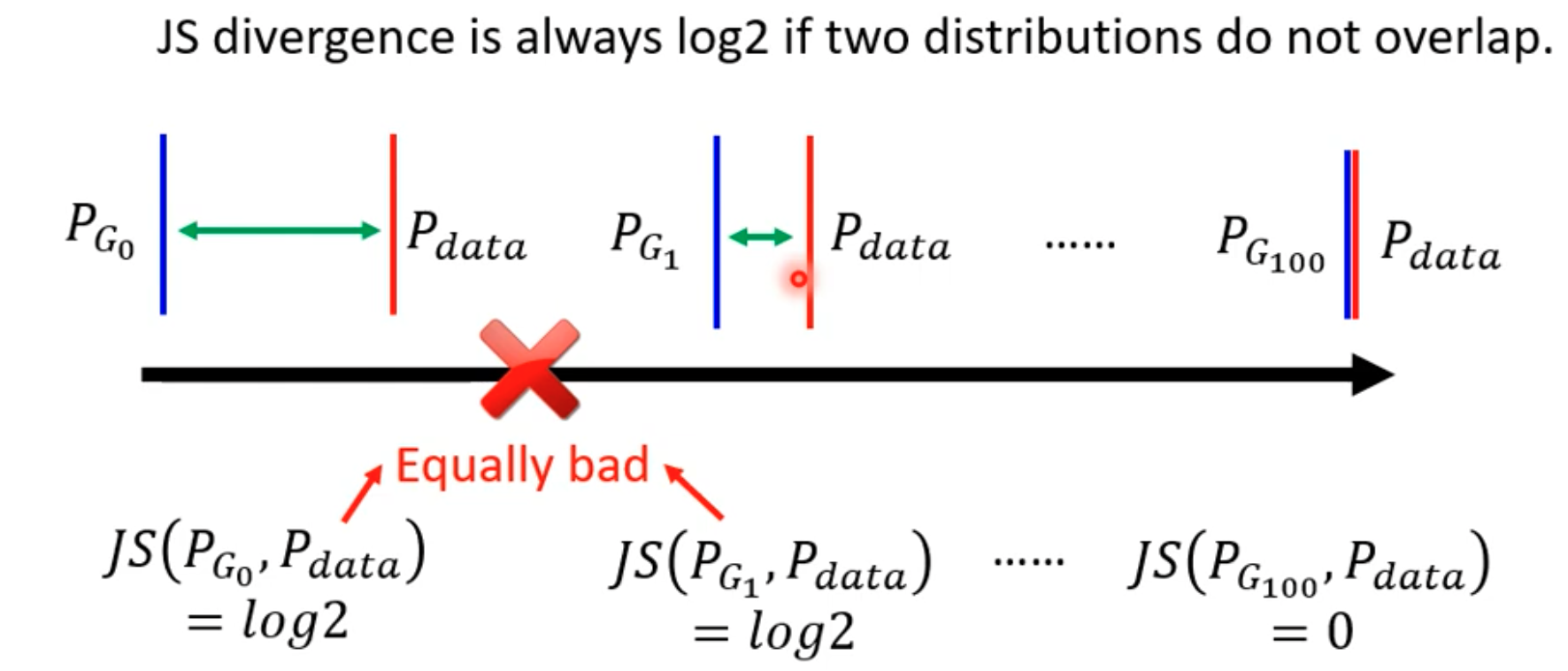
A binary classifier can easily distinguish generated images from real images, so the objective $\max_D V(D,G)$ remains large and cannot effectively represent the JS distance.
Therefore, we can switch to other distances, such as Wasserstein distance, so that the distance can reflect the relative distance between $P_g$ and $P_{data}$.
In addition, during GAN training, both the generator and discriminator are expected to converge. Once one side has a problem, the other side cannot train normally. However, in ordinary training, it is common for a loss to increase instead of decrease. Therefore, we need the generator and discriminator to remain well matched.
Generating text with GAN is among the most difficult tasks. When the generator decoder produces text, the discriminator scores the text. If the generator is updated and a parameter changes, the final text token is usually obtained through an argmax operation. The argmax result may not respond smoothly to parameter changes. That is, the final text judged by the discriminator may remain unchanged, so the score is the same, making training difficult. One possible solution is to use reinforcement learning for training.
Other generative models include VAE and flow-based models.
GAN Evaluation
Evaluating the quality of generated images:
Human evaluation.
Use a face recognition model or image classification model to judge the quality of generated images.
- Mode collapse: generated images look realistic, but they are all very similar to one particular real image.
- Mode dropping: the generated image distribution covers only part of the real image distribution, or the generated images only focus on some characteristics of real images.
Image generation metrics: quality and diversity.
For generation diversity, use a classification model to classify generated images and check whether the predicted labels are evenly distributed.
Evaluation metrics:
- Inception Score: use an Inception model for classification and evaluate quality and diversity.
- Frechet Inception Distance (FID): use the hidden-layer vector before the softmax layer of an Inception network to represent the current image. Assuming real and generated image features follow Gaussian distributions, compute the Frechet distance between their feature distributions.
Extreme cases may also occur, such as the generator directly generating original images or inverted images.
Conditional Generator
The generators discussed above all take a randomly sampled $z$ as input and generate the desired output. Now we add an input $x$ to the generator to control its output.
Text-to-image generation is one such task.
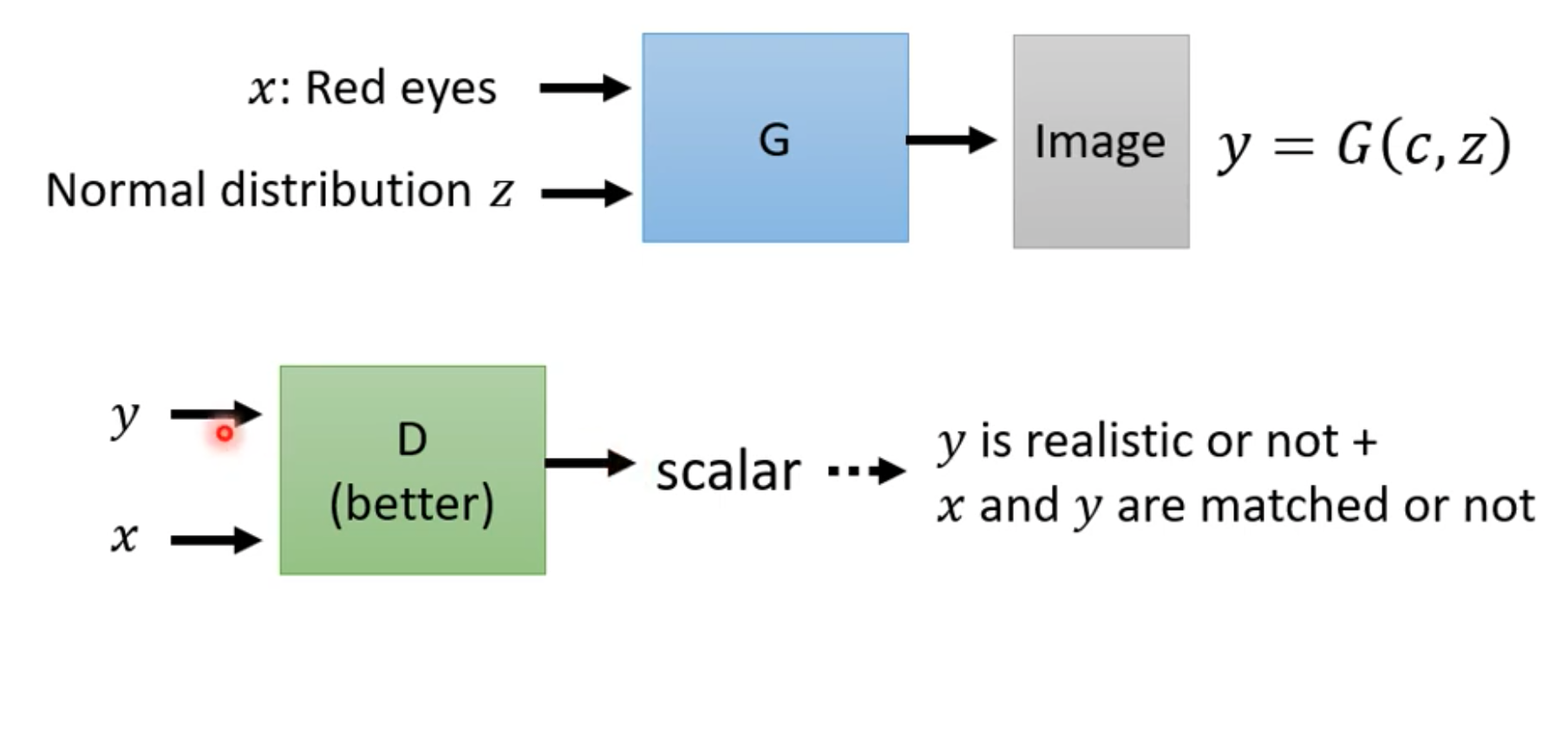
This kind of conditional generator also requires redesigning the discriminator, so that the discriminator reads the condition $x$ as well.
Such a discriminator requires paired labeled training data:
- real image and text pairs are labeled as 1;
- input text and generated image pairs are labeled as 0;
- mismatched input text and real image pairs are also labeled as 0.
Conditional GANs can also be used for image-to-image generation and related tasks.
For image-to-image generation, if we only use a supervised model, the model may face the same issue mentioned at the beginning: multiple outputs can all be correct. The model may learn to average these possibilities, resulting in blurry generated images. Using an adversarial generative model can help avoid this situation.
This kind of conditional GAN requires paired labeled data.
GANs in Unsupervised Learning
In image style transfer, there is no paired data for training.
Suppose we want to translate real photos into anime-style images. We are given real photos from domain $X$ and anime images from domain $Y$. Note that the anime images and real photos have no one-to-one correspondence; both may simply be images collected from the internet.
By analogy with ordinary GAN:
- Treat real-photo domain $X$ as a distribution, sample from it as input to the generator, let the generator produce an image, and let the discriminator compare the generated image with anime images.
- The problem is that the generated image and anime image still have no correspondence during training. In an extreme case, for an input real image, the generator could simply find any anime image as its output, and the discriminator could still be trained very well.
CycleGAN:
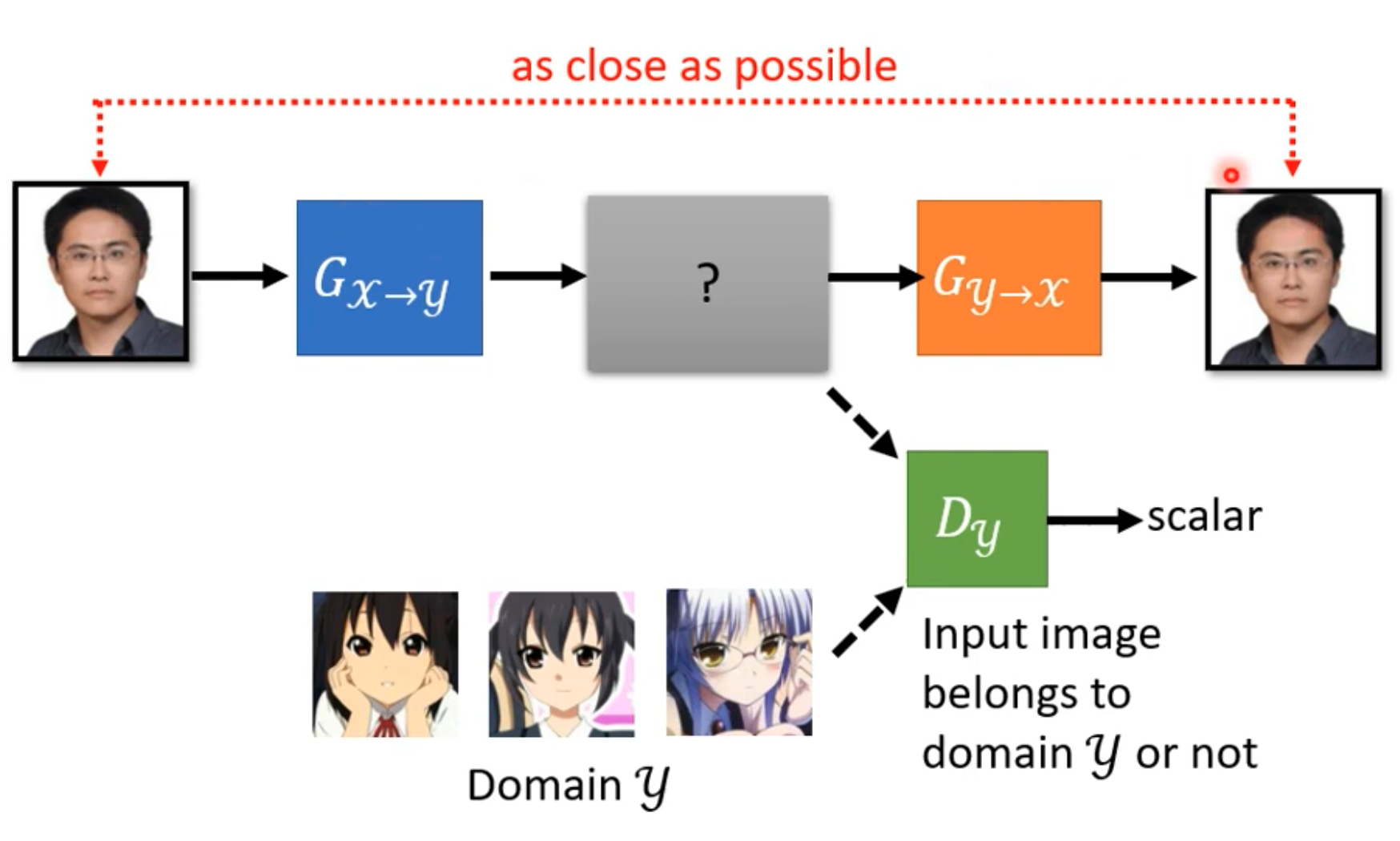
It contains three models. The first generator cannot freely generate arbitrary anime images. A second generator must map the generated image back to the real-image domain. In this way, the relationship between real images and anime images can be learned.