Previously, whether we discussed self-supervised learning or autoencoders, the essence was still that the machine recognized labels. In this sense, they still belonged to the supervised-learning paradigm.
Reinforcement learning usually faces a different scenario: humans may not know what the exact label should be, or how to evaluate whether a label is good or bad, but the machine still needs to know the criteria for judging good and bad behavior.
1. What Is RL
In essence, reinforcement learning is similar to supervised learning in that it also tries to find a function. The input is the observed change in the environment, or observation, and the output is an action to take. During this process, the environment gives this function a reward, telling it whether the current action is good or bad. The goal is to maximize the total reward obtained over time.
The three simplified steps of machine learning are:
- There is a function with unknown parameters.
- A loss function is defined from the training data.
- The unknown parameters of the function are optimized so that the loss is minimized.
By analogy, the simplified steps of reinforcement learning are:
There is also a function with unknown parameters.
It plays the role of the actor and is called the policy network.
Before deep learning, it could also be a simple rule-based method. Today, most policy networks are deep networks.
Its input is the observed state, and its output is the score or softmax probability of each possible action. In essence, this resembles a classification task.
Finally, the action is sampled according to the scores of all possible actions. Here, sampling means randomly producing an action.
Define the loss.
- During a whole game, from the first step to the end, every action taken by the machine receives a reward.
- The process from the beginning to the end of a game is called an episode, and the sum of rewards over all steps is called the total reward.
- The loss can be regarded as the negative total reward. The training objective is to maximize the total reward.
Optimize.
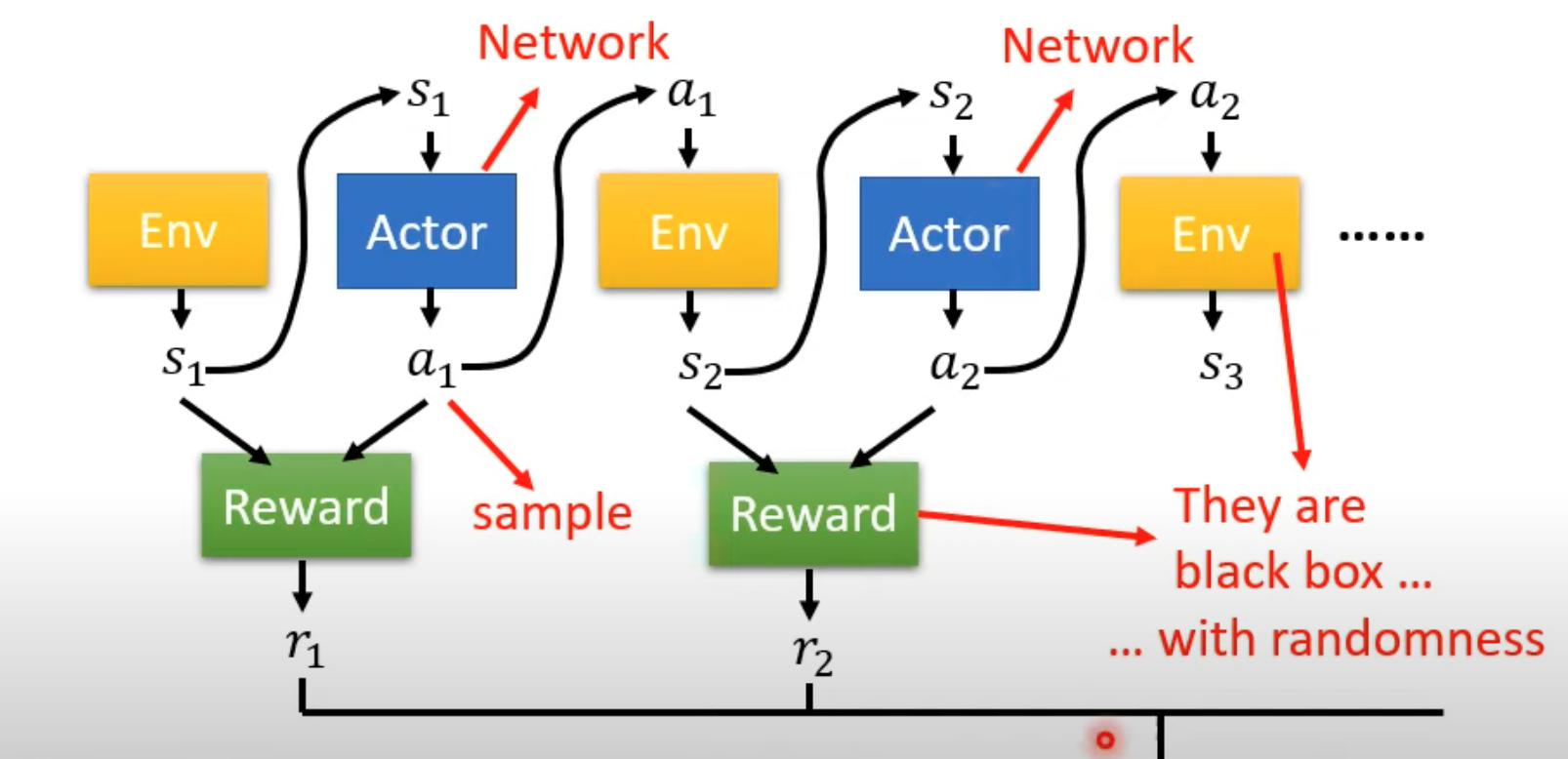
The whole learning process contains three modules. The actor is the network we want to train. The environment provides the current state as the network input. The reward module provides the reward after the system takes an action.
As the game proceeds, the actor generates a trajectory:
$$ \tau=\{s_1,a_1,s_2,a_2,\ldots,s_n,a_n\} $$After each action, a reward $r_i$ is produced. The optimization goal is to maximize the sum of all rewards.
If we view the entire process as a sequence, we might think about using sequence models such as RNNs to optimize the maximum reward. However, this is not easy to train because:
- The actor has randomness when taking actions. It may not always choose the action with the highest score.
- The environment, actor, and reward cannot be treated as one complete trainable system. The environment and reward are not necessarily neural networks. To us, they are black boxes, and we do not know their internal parameters.
- The environment or reward can also be stochastic in some scenarios. For a certain state and action, the next state of the environment may not be deterministic.
From these aspects, RL and GAN have something in common:
- In GAN, we can connect $D$ and $G$, fix $D$, and train $G$. In RL, we can view the actor as $G$, and view the environment and reward as $D$. The loss of RL comes from the reward output, while the loss of GAN comes from the discriminator output. By analogy, we can think of connecting the actor with the environment and reward for training.
- However, unlike GAN, the environment and reward are black boxes, not neural networks, so they cannot be optimized directly.
2. Policy Gradient Optimization
Start by training an actor. Treat the actor’s task as a simple classification or regression task: given a state, output the probability of taking each possible action. For now, ignore randomness, and assume all possible action categories are known.
For such an actor, the loss can be cross-entropy: $L=\sum e$. If, for a certain state, we do not want the actor to take a certain action, while allowing it to take other actions, we can use negative cross-entropy: $L=-\sum \hat{e}$.
For this classification problem, we can use a loss function such as
$$ L=\sum e-\sum\hat{e} $$The required training data is $\{s_i,\hat{a}_i\}, 1\ \text{or}\ -1$, which means that in state $s_i$, the system should take action $\hat{a}_i$, or should not take action $\hat{a}_i$.
The training data above forms a binary classification problem. Going further, if we want to specify how desirable it is to take action $a$, we can view the problem as a regression task. This is not exactly the same as traditional regression, because the action category and its desirability are both involved. The training data becomes $\{s_i,\hat{a}_i\},A_i$, meaning that the desirability of taking action $\hat{a}_i$ in state $s_i$ is $A_i$. The corresponding loss can be written as $L=\sum A_i e_i$.
Therefore, in essence, optimizing the actor can be viewed as training a classification or regression model, except that the training data must be specially determined. In practice, however, the specific action $a_i$ in the training data is not easy to obtain. This is a key point of reinforcement learning.
1. How to Obtain the Training Behavior $\hat{A}_i$
The key to obtaining RL training data is how to evaluate each state-action pair with a score $A$.
First, randomly initialize the actor with parameters $\theta_0$.
For each training episode:
Use the actor to obtain a sequence of $\{s_i,a_i\}$ data.
Use some method to compute the desirability score $A_i$ of each state-action pair.
Use the data from the current episode to compute the loss.
Perform one gradient descent update:
$$ \theta^i=\theta^{i-1}+\eta\frac{\partial L}{\partial \theta^{i-1}} $$
Important points:
- A sequence of training data is generated only within each episode. That is, the training data does not exist from the beginning; it is produced during each episode.
- In each episode, the parameters can only be updated once, and the update can only use the training data from the current episode. This is because the training data of the $i$-th episode is generated by the actor with parameters $\theta^i$, and is only related to $\theta^i$, not to $\theta^{i-1}$.
Therefore, RL training is time-consuming and difficult. Here, an episode simply means completing one round of the game.
The key issue in the whole training process is how to obtain $A_i$ for the data pairs from the reward or environment. If $A_i$ needs to accumulate future rewards, we may need to finish the current game and then compute $A_i$ backward for each step.
Several ideas are possible:
Directly use the reward of $\{s_i,a_i\}$ as $A_i$.
- The current action affects not only the current moment, but also the future.
- Reward delay problem: the current action may only take effect later and lead to a high reward. Therefore, receiving a low current reward does not necessarily mean the current action is bad.
Cumulated reward: use the sum of all rewards from the current action to the end as $A_i$:
$$ A_i=\sum_{k=i}^N R_k $$If the game is very long, the current action may have little relationship with the final reward.
Therefore, weights can be added, giving the discounted cumulated reward:
$$ G_i=\sum_{k=i}^N \gamma^{k-i} R_k,\quad \gamma=0.9 $$Reward is relative. Even if all rewards are positive, they still need to be compared relatively.
Add a baseline to every $A_i$ to avoid all values being positive:
$$ A_i=\sum_{k=i}^N R_k-b $$
Note: $G$ and $A$ above are not exactly equivalent. $A_i$ refers to the expected quality of an action, while $G_i$ refers to the accumulated future reward. Whether $G_i$ is positive or negative represents whether the reward is positive or negative; the absolute sign is not important, because it should be interpreted relatively. By contrast, $A_i$ is an evaluation criterion. If $A_i>0$, the current action is good; if $A_i<0$, the current action is poor.
2. Off-Policy
The training process described above, where the model trains while interacting with the environment, is called on-policy training.
Another approach is to collect all interaction state-action pairs at once and then directly use them during training. This is called off-policy training.
- The actor to be trained uses state-action pairs collected from interactions between another actor and the environment.
- In other words, the data is collected once and used repeatedly for training.
A classic off-policy training strategy is Proximal Policy Optimization (PPO). Its main idea is to make the actor being trained aware of the gap between itself and the actor that generated the training data.
3. Actor-Critic
Using a critic also requires training a suitable critic, just as we previously trained the actor.
The critic is used to predict how good the discounted cumulated reward may be for the current actor under a certain state $s$.
Essentially, the critic is a value function $V^\theta(s)$. Its input is the current state $s$, and it estimates the cumulative reward that the actor with current parameters $\theta$ may obtain until the end of the game:
$$ G_i=\sum_{k=i}^N \gamma^{k-i}R_k,\quad \gamma=0.9 $$The output is an expected value. Therefore, the critic’s job is to predict the future: by looking only at the current state, it estimates the reward that may be obtained in the rest of the game.
The critic needs to observe the current actor, and it should match the actor with the current parameter $\theta$. If the actor with current $\theta$ performs poorly, then the critic’s estimated cumulative reward should also be relatively small.
With actor-critic, we can improve the computation of $A_i$ described above.
1. Training Methods for the Critic
Monte Carlo method.
- Let the actor with current parameter $\theta$ interact with the environment and complete multiple games, producing a batch of training data. These data contain all states $s$, and we can obtain the accumulated reward $G'$ for every state.
- The training method is to make the critic’s output $V^\theta(s)$ for state $s$ as close as possible to the actual $G'$ of that state.
Temporal-difference (TD) method.
The Monte Carlo method above requires complete games in the collected training data, but in many cases finishing a whole game can be costly. TD methods can train the critic without completing the entire game.
TD requires interactions from the current actor and obtains a sequence of training data:
$$ \ldots,\{s_t,a_t,r_t\},\{s_{t+1},a_{t+1},r_{t+1}\},\ldots $$Observe the computation of $V^\theta(s_t)$:
$$ V^\theta(s_t)=r_t+\gamma r_{t+1}+\gamma^2 r_{t+2}+\cdots $$$$ V^\theta(s_{t+1})=r_{t+1}+\gamma r_{t+2}+\gamma^2 r_{t+3}+\cdots $$$$ V^\theta(s_t)=r_t+\gamma V^\theta(s_{t+1}) $$According to the relationship between $s_t$ and $s_{t+1}$, we hope the training data satisfy
$$ V^\theta(s_t)-\gamma V^\theta(s_{t+1}) \approx r_t $$
The two methods above may train different critics for the same state $s$ even when using the same training data.
When training the critic, the sampled training data should cover as many states as possible, as well as all possible actions under those states.
2. Role of the Critic
With the critic, we can compute $\hat{A}_i$ more effectively.
Based on the previous methods for computing $\hat{A}_i$, we can continue improving with the critic:
For $\{s_t,a_t\}$, let
$$ A_t=G'_t-V^\theta(s_t) $$- For method 3, $A_i=\sum_{k=i}^N R_k-b$, the value of $b$ is hard to determine. A better idea is to set $b=V^\theta(s_i)$.
- In this case, $A_i$ can evaluate how good or bad it is to take a certain action in the current state. Here, $V^\theta(s_t)$ is the average expectation over all possible actions.
- The reason this is better is that $V^\theta(s_t)$ represents the expected accumulated reward that can be obtained from the current state $s_t$.
- Moreover, in state $s_t$, the actor does not necessarily execute action $a_t$. The value $V^\theta(s_t)$ includes the expectation over all possible actions that may be taken from $s_t$. Recall that the actor was designed to output a probability distribution over actions, and we hope it has randomness in action selection, perhaps the more randomness the better. Therefore, $V^\theta(s_t)$ represents the expected reward of taking all possible actions.
- Thus, for $\{s_t,a_t\}$, $A_t=G'_t-V^\theta(s_t)$. Here, $G'_t$ represents the accumulated reward obtained by taking action $a_t$ in state $s_t$, while $V^\theta(s_t)$ represents the expected accumulated reward over all possible actions in state $s_t$. If $A_t>0$, then taking action $a_t$ is better than the average effect of all actions; otherwise, the reward of the current action is lower than that of randomly taking actions.
For $\{s_t,a_t\}$, let
$$ A_t=r_t+V^\theta(s_{t+1})-V^\theta(s_t) $$- Let $r_t+V^\theta(s_{t+1})=G'_t$.
- In method 4, $V^\theta(s_t)$ is a statistical value, while $G'_t$ is an exact value obtained from one training episode. Replacing $G'_t$ with a statistical value can be more effective.
- Simply speaking, $G'_t$ represents the accumulated reward obtained by taking action $a_t$ under state $s_t$, while $V^\theta(s_t)$ represents the average expected accumulated reward from all possible actions under state $s_t$.
- Therefore, for state $s_t$, the statistical value of $G'_t$ can be expressed using the statistical value of the next state $s_{t+1}$ and the reward $r_t$ obtained by taking action $a_t$.
- At this point, $A_t$ indicates whether taking action $a_t$ in state $s_t$, receiving $r_t$, and then taking random future actions is better or worse than randomly taking actions from the current state $s_t$.
- This is the well-known Advantage Actor-Critic method.
- In concrete training, we can share some parameters between the actor and the critic. The actor outputs a distribution over different actions, while the critic outputs the value of the accumulated reward.