Understanding Variational Autoencoders

Autoencoder

General Architecture of Autoencoders

The concept of an autoencoder was originally proposed for dimensionality reduction. Given an original feature vector $x$, we hope to obtain a low-dimensional representation $e(x)$ that still preserves rich information from the original features through selection, combination, transformation, and related operations. Usually $|e(x)|\ll|x|$. This type of learning is also called representation learning.

Intuitively, unlike supervised learning, we cannot predefine the desired low-dimensional representation for every feature. Therefore, we need a self-supervised method to discover relationships among the original features. There are many ways to perform representation learning. Here, we follow one class of dimensionality-reduction methods based on the Encoder-Decoder architecture. This architecture uses an encoder to compress the original features into a low-dimensional code, and then uses a decoder to reconstruct the input from that code. In this way, we construct a self-supervised learning task whose objective is to make the reconstruction as close as possible to the original input.

The low-dimensional code can be regarded as an information bottleneck: important information in the original features should be able to pass through this bottleneck and still be reconstructed.

preview

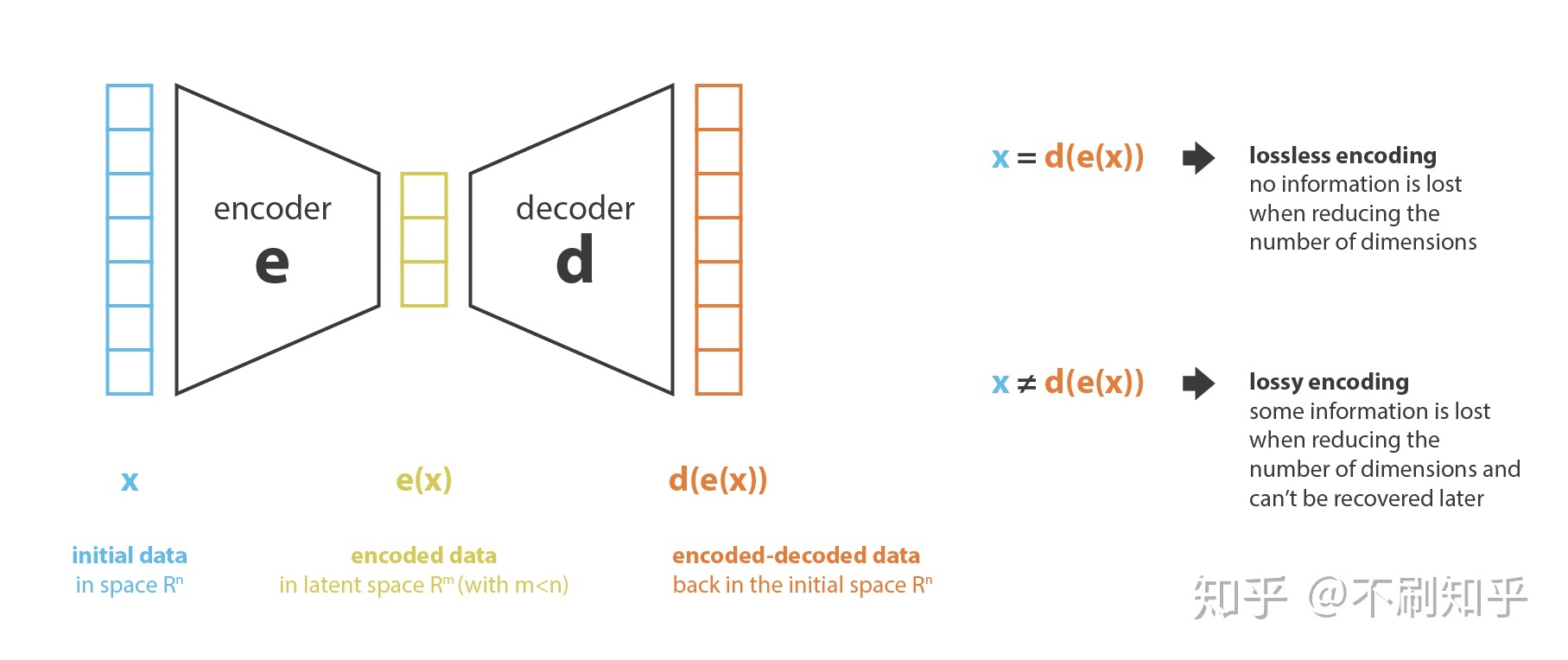
In general, a dimensionality-reduction problem can be written as:

$$ \begin{aligned} e,d &= \operatorname*{arg\,min}_{(e,d)\in E\times D} \operatorname{Loss}\left(x,d(e(x))\right) \end{aligned} $$

PCA for Dimensionality Reduction

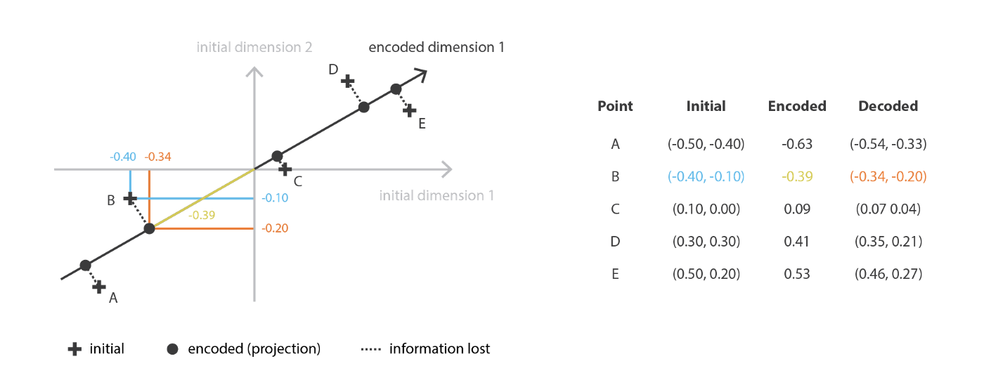
When people talk about dimensionality reduction, the first method that often comes to mind is the well-known PCA, or Principal Component Analysis. Its core idea is to identify the main directions of variation through singular value decomposition (SVD), and then project the original features into a lower-dimensional representation space through linear combinations.

I will not go into the detailed derivation of PCA here, but its main procedure can be placed into the autoencoder framework. In PCA, the encoder and decoder correspond to the projection matrix $W$ and its transpose $W^T$.

Deep Autoencoder

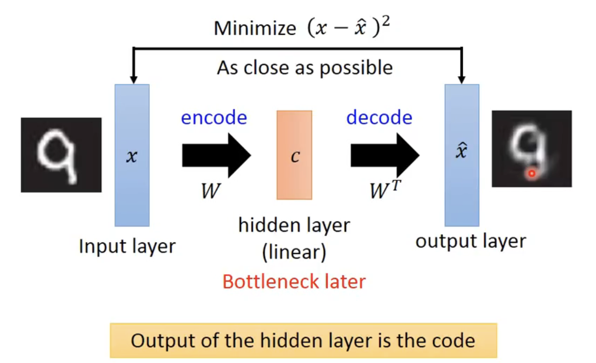
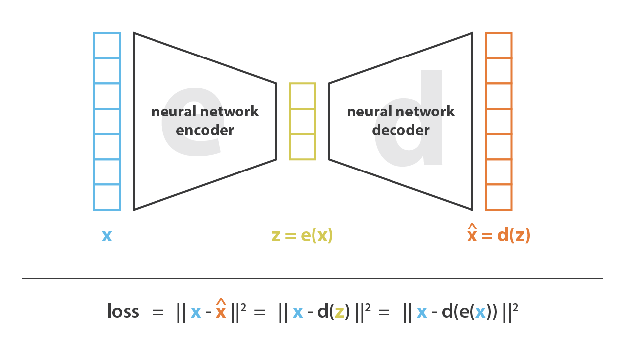
The key to an autoencoder lies in the mapping functions of the encoder and decoder. Therefore, a natural idea is to use the strong fitting ability of neural networks to construct the encoder and decoder directly. During each iteration, we compare the decoder output with the original input and update the network weights through backpropagation.

This idea was proposed by Hinton in the 2006 paper published in Science, which also released the code at that time. It is worth noting that Hinton had already pointed out that this autoencoder architecture could be used to build unsupervised tasks for pre-training, followed by fine-tuning on real data. Therefore, in essence, the idea of pre-training is to construct an appropriate unsupervised task, which is the most important part, to initialize model parameters effectively. Then, with only a small amount of supervised fine-tuning, the model can obtain strong performance.

It is useful to revisit the main idea from that paper. The authors showed that a deep network with a narrow middle layer can learn compact codes by reconstructing high-dimensional inputs. They also emphasized that gradient-based fine-tuning works much better when the initial weights are already close to a good solution, which motivated their pre-training strategy.

Compared with PCA, the greatest advantage of neural networks is that their feature mappings can be nonlinear, which cannot be achieved by ordinary matrix transformations alone. In other words, if we use a simple neural network without nonlinear transformations, that is, without activation functions, the neural network can simulate the linear transformation behavior of PCA. In theory, a deep nonlinear neural network can compress features into a sufficiently small latent space while reconstructing the low-dimensional features without information loss. In Hinton’s paper, for the MNIST dataset, each image with 784-dimensional features could be compressed into 30 dimensions and reconstructed clearly, which was quite impressive at that time.

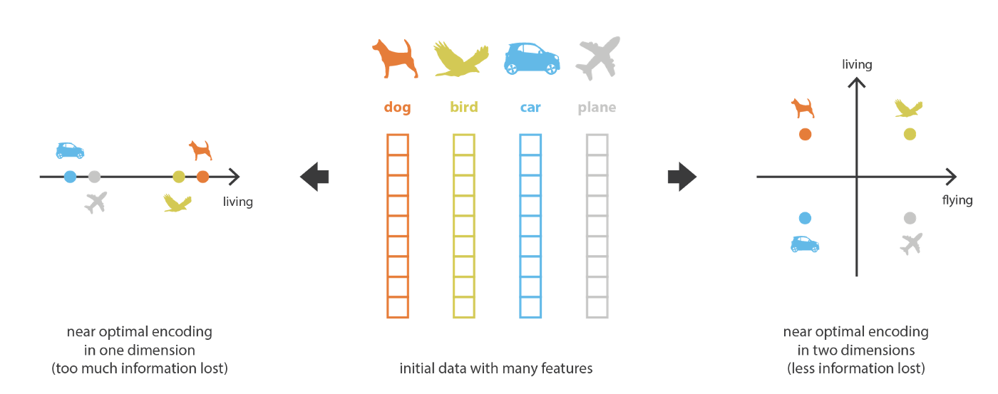
However, we cannot shrink the information bottleneck indefinitely. Although an extremely low-dimensional code may still be reconstructed by a powerful decoder, the decoder is then more likely to memorize the data codes. In that case, the intermediate code inevitably loses a great deal of important information, as shown in the following figure. The one-dimensional representation on the left only preserves whether the object is biological, while the two-dimensional representation on the right separates biological identity and flying ability into two dimensions.

An overly low-dimensional latent space lacks interpretable and useful structure, or in other words, it has a lack of regularity. Therefore, the goal of dimensionality reduction is not to make the information entropy as low as possible, but to reduce dimensionality while preserving the main structural information of the data in a simplified representation. For these reasons, the size of the latent space and the “depth” of the autoencoder, where depth refers to the degree and quality of compression, must be carefully controlled according to the final purpose of dimensionality reduction.

As the name suggests, the original motivation of autoencoders is to obtain low-dimensional representations of the features of original objects. Such low-dimensional representations can be used in many scenarios:

Text retrieval: obtain document word vectors and reduce their dimensionality; represent a query in the reduced space and retrieve documents according to distances in that space.
Image retrieval: instead of measuring pixel-level distances, reduce the dimensionality of both the query image and the candidate images, and evaluate image similarity using distances in the low-dimensional space.
Pre-training of model weights.
And so on.

In these scenarios, our focus is on the encoder, while the decoder only serves as an auxiliary structure during training. However, when studying generative models, we need to focus on the decoder, because it is the main component responsible for generating the target output. Due to the original purpose and limitations of autoencoders, it is relatively difficult to directly modify a standard autoencoder for image generation. A successful direction along this line is the variational autoencoder, or VAE, which we will discuss next.

In my own view, the inherent limitations of the autoencoder architecture still constrain the expressive power of VAEs today, because autoencoders were not originally born for generative modeling.

Variational Autoencoder

For a variational autoencoder, the key component is the decoder. The goal is to construct a generative model: given a vector code sampled from a certain distribution, the model should generate an output that follows a certain “form”. This “form” is learned in a self-supervised way from the given dataset through the cooperation of the encoder and decoder.

The VAE was introduced in Auto-Encoding Variational Bayes. The original goal of the paper was to propose a gradient-estimation method called Stochastic Gradient Variational Bayes, using neural networks for variational inference and parameterizing the variational distribution. A plain explanation is that we want to construct a distribution $q(x,\theta)$ to approximate an intractable distribution $p(x|z)$, and we directly use a neural network to build this $q(x,\theta)$. Along the way, the authors proposed the Variational Bayes Auto-Encoding algorithm, namely the VAE framework.

The main motivation of the original paper can be summarized as follows: how can we perform efficient inference and learning in directed probabilistic models when continuous latent variables, intractable posterior distributions, and large datasets appear at the same time? The paper answers this by introducing a scalable stochastic variational inference method.

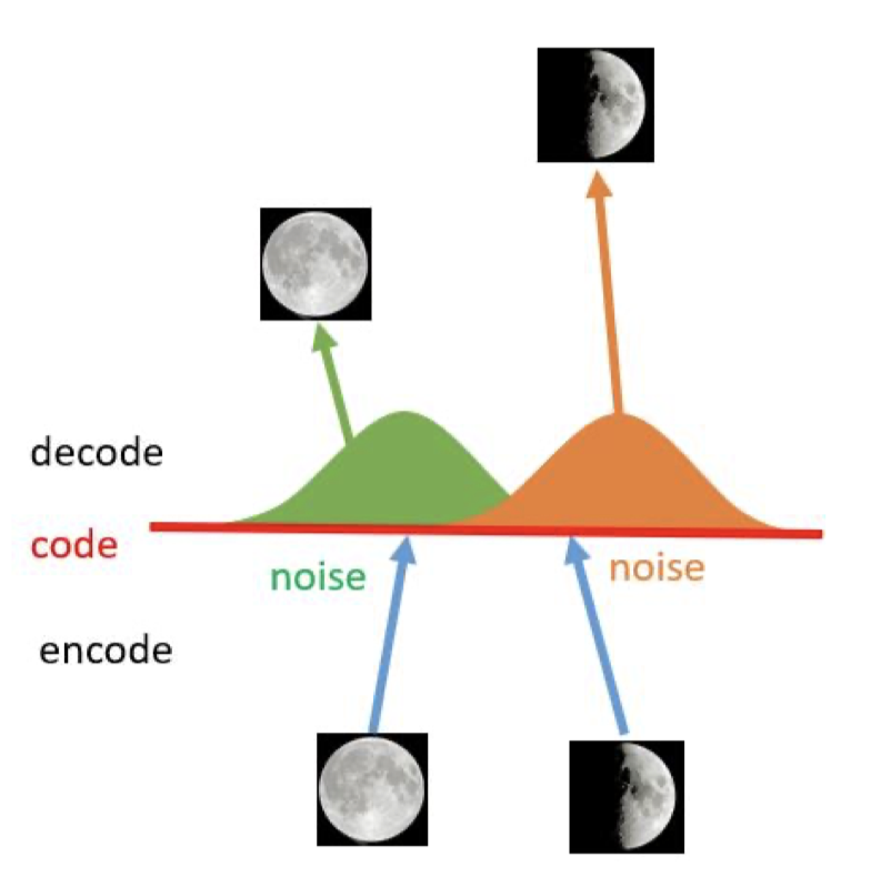
Of course, the structure of a VAE comes from the autoencoder, but their objectives are different. We should not simply reason by analogy. Although an ordinary autoencoder also has a process of generating an output from a code $z$, it cannot be directly used as a generative model. The reason is that the codes learned by an autoencoder are overfitted in the latent vector space. More specifically, the codes of similar inputs can be discrete in the latent space and may not support linear transitions. In other words, the encoder and decoder have “rigidly” memorized different codes, but there is no close relationship between the codes themselves.

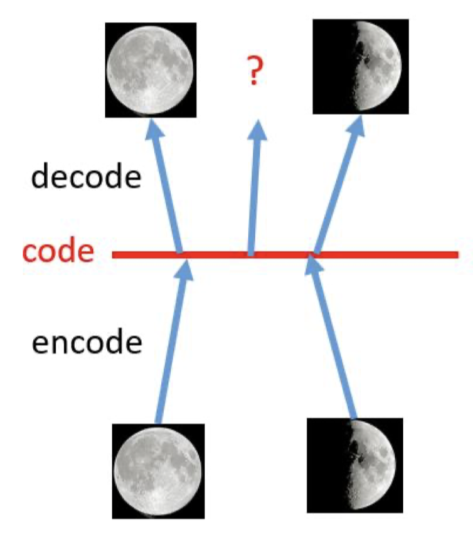
As shown above, for the codes of a full moon and a half moon, the decoder can reconstruct the original images accurately. However, if we sample from the linear region between the two codes, the decoder cannot produce a meaningful result from the intermediate code. That means it does not really have generative ability.

Fundamentally, this happens because the loss of an autoencoder only depends on the difference between the generated result and the original data; it does not care how the code vectors are organized in the latent space. If we can also make code regularization part of the learning objective, then the decoder can decode samples from continuous regions in the latent space, instead of being limited to discrete code points. Intuitively, we want to generalize the coding space of the data so that it does not overfit to specific discrete codes. This is the process of regularizing the codes.

To generalize the codes, one first possible idea is to add noise to the original image. This can make the encoder map inputs into a local region, but it is still not sufficient. The clever part of VAE is that it uses a distribution to represent the code of each data point, thereby turning an originally discrete code into a kind of continuous code. The following paragraphs explain what this means.

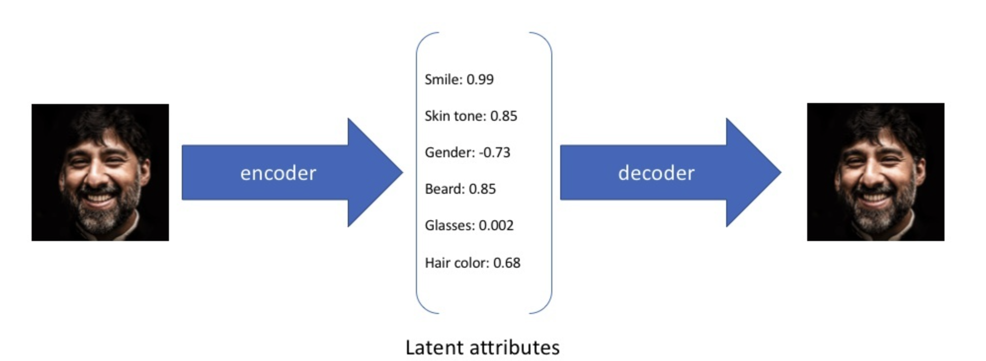
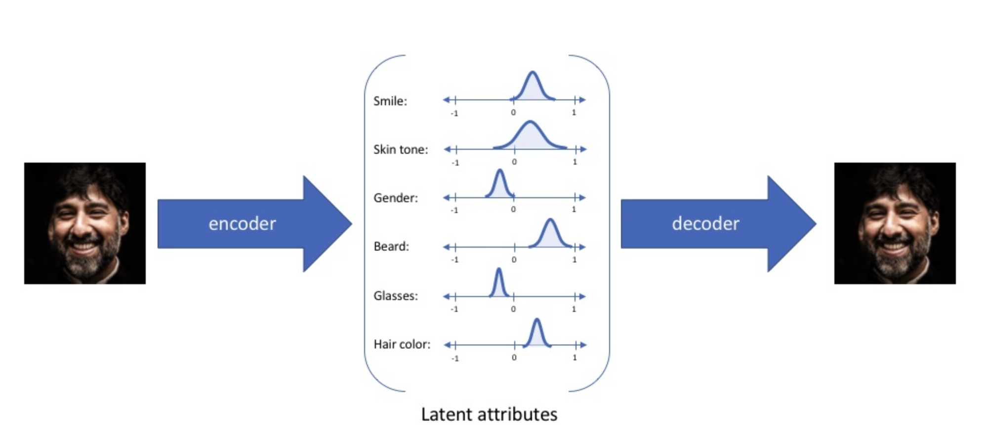
When using a VAE as a generative model, we hope that a latent vector $z$ randomly sampled from the code space can always produce an approximate generated result, and the closer it is to the original image’s code, the more similar its features should be to the original image. What VAE does is to turn a discrete code, such as $z=[2,4,3,6]^T$, into the form of a continuous function, such as $Z=\mathcal{N}(\mu,\sigma^2),\mu,\sigma^2 \subset \mathbb{R}^n$, as shown above.

After obtaining a code distribution, we randomly sample from it to obtain a code vector $z=rand(Z)$. In theory, codes sampled from this distribution should contain some information from the original data, and the position near the mean contains the most information. The advantage is that codes in the overlapping region of two distributions contain common features of the two data points. In this way, continuity of the code is achieved. VAE training is regularized to avoid overfitting and to ensure that the latent space has desirable properties for data generation.

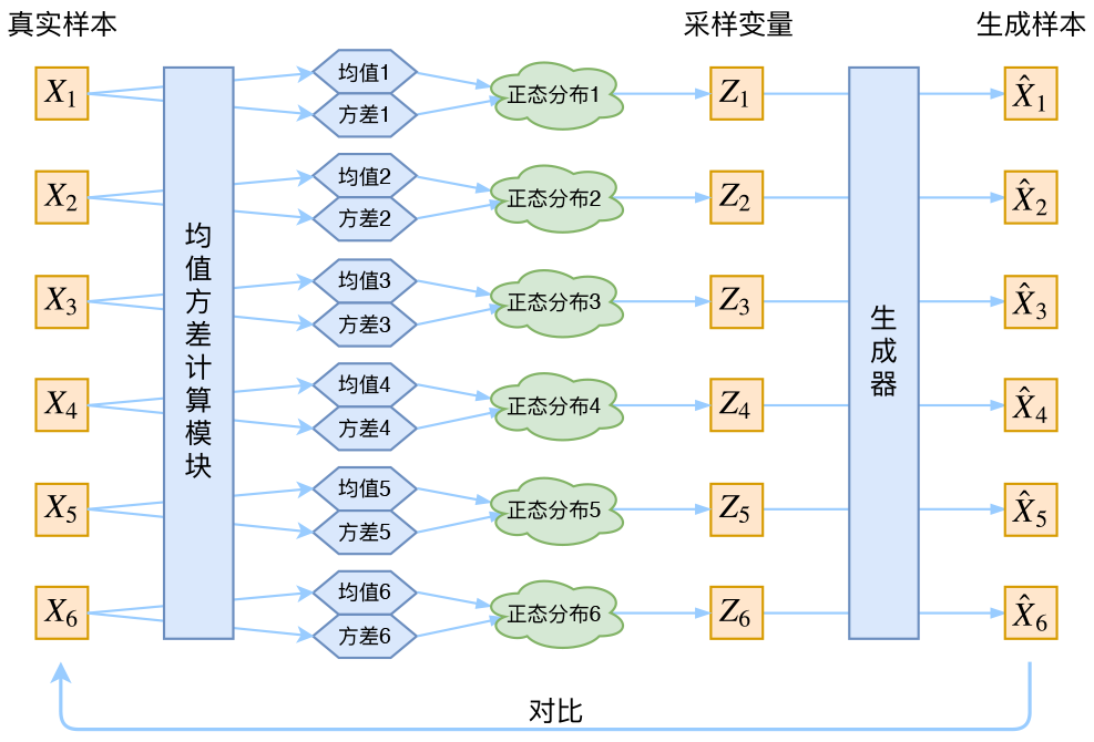
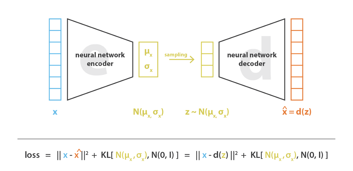
As shown above, we usually use a normal distribution for the code. In practice, to represent a normal distribution, we need its mean $\mu$ and variance $\sigma^2$. Note that $\mu,\sigma^2 \subset \mathbb{R}^n$ are both multidimensional variables. From this perspective, the actual job of the encoder in a VAE is to construct the mean and variance of the distribution for the input data.

For each input data point $x_i\in X$, there is a dedicated corresponding normal code distribution. From the encoder’s perspective, $\mu_i,\sigma_i^2 = e(x_i) \subset \mathbb{R}^n$. From the perspective of the input data point $x_i$, its dedicated distribution is $p(z|x_i)=\mathcal{N}(\mu_i,\sigma^2_i)$. Therefore, the complete VAE architecture is shown below.

Encoding Details

Now that we know VAE uses a normal distribution to encode each data point, the next question is: how can the model learn the relationship between data and distributions?

From the analysis above, since we use a distribution as the code, and the code distribution $p(z|x)$ is assumed to be a normal distribution as prior knowledge, the encoder can directly output the two parameters of the distribution corresponding to that data point: the mean $\mu$ and the covariance matrix $\sigma^2$. In other words, we can construct two neural networks, $\mu_i=f(x_i)$ and $\log \sigma_i^2=g(x_i)$, to approximate these two parameters.

The reason we fit $\log \sigma^2_i$ instead of $\sigma_i^2$ is that $\log \sigma^2_i$ can be either positive or negative, while $\sigma_i^2$ must be positive and would require special handling through an activation function. From the perspective of the normal distribution, the fitted mean and variance ensure local and global regularization of the latent space, respectively: the variance controls local regularization, while the mean controls global regularization.

After this treatment, when we look again at the VAE architecture above, we can see two main differences from the original autoencoder. First, there is an additional encoding output, which encodes the variance $\sigma^2$. Second, the code $z$ is sampled from a distribution.

The second difference is what gives VAE its generative ability. Because $z$ is not obtained directly from the encoder, we want the output $\hat{x_i}$ generated from the sampled $z$ to remain as close as possible to the original input $x_i$. The sampling process is essentially a process of adding noise: the complete code $\hat{z}$ is the mean, while the sampled $z$ deviates from $\hat{z}$. For now, we ignore the difficulty of backpropagation caused by sampling.

Adding noise increases the difficulty of reconstruction. However, as discussed above, the mean and variance can ensure regularization of the latent coding space. More directly, the variance controls the strength of the noise: a smaller variance keeps samples closer to the mean. Since the variance is computed by the encoder neural network, if the network wants to maximize reconstruction quality, it will tend to reduce the noise as much as possible. In other words, the network will try to make the variance approach zero. In that case, the code distribution loses randomness, and no matter how we sample, we obtain the result at the mean. The model then degenerates into a basic autoencoder, and the variance code no longer plays any role.

How do we solve this noise-collapse problem? We add a regularization constraint on the encoder to the learning objective, forcing all code distributions to align with the standard normal distribution. I also really want to know how this idea was originally discovered. This prevents the noise from becoming zero and also preserves the model’s generative ability.

Why can a standard normal distribution help guarantee generative ability? Our goal is to make the code distribution $p(z|x_i)$ close to the standard normal distribution $\mathcal{N}(0,1)$. According to the definition:

$$ \begin{aligned} p(z) &= \sum_{x_i\in X}p(z\mid x_i)p(x_i) \\ &= \sum_{x_i\in X}\mathcal{N}(0,1)p(x_i) \\ &= \mathcal{N}(0,1)\sum_{x_i\in X}p(x_i) \\ &= \mathcal{N}(0,1) \end{aligned} $$

Therefore, when we use the decoder directly to generate results, we can randomly sample $z=rand(p(z))$ from the normal distribution, and any code $z$ can generate a result with specific information.

To make every code distribution align with the normal distribution, we can add a KL divergence term to the loss function to measure the distance to the normal distribution. The closer the code distribution $p(z|x_i)=\mathcal{N}(\mu_i,\sigma^2_i)$ is to the normal distribution $\mathcal{N}(0,1)$, the smaller the KL divergence will be.

As shown in the figure above, the learning objective of VAE contains two parts: the reconstruction term $||x-\hat{x}||^2$, and the regularization term $KL(\mathcal{N}(\mu_i,\sigma^2_i),\mathcal{N}(0,1))$. The former optimizes the encoder-decoder structure, while the latter regularizes the code space.

Let us think more carefully about why we need regularization, and why the code distributions should align with a normal distribution.

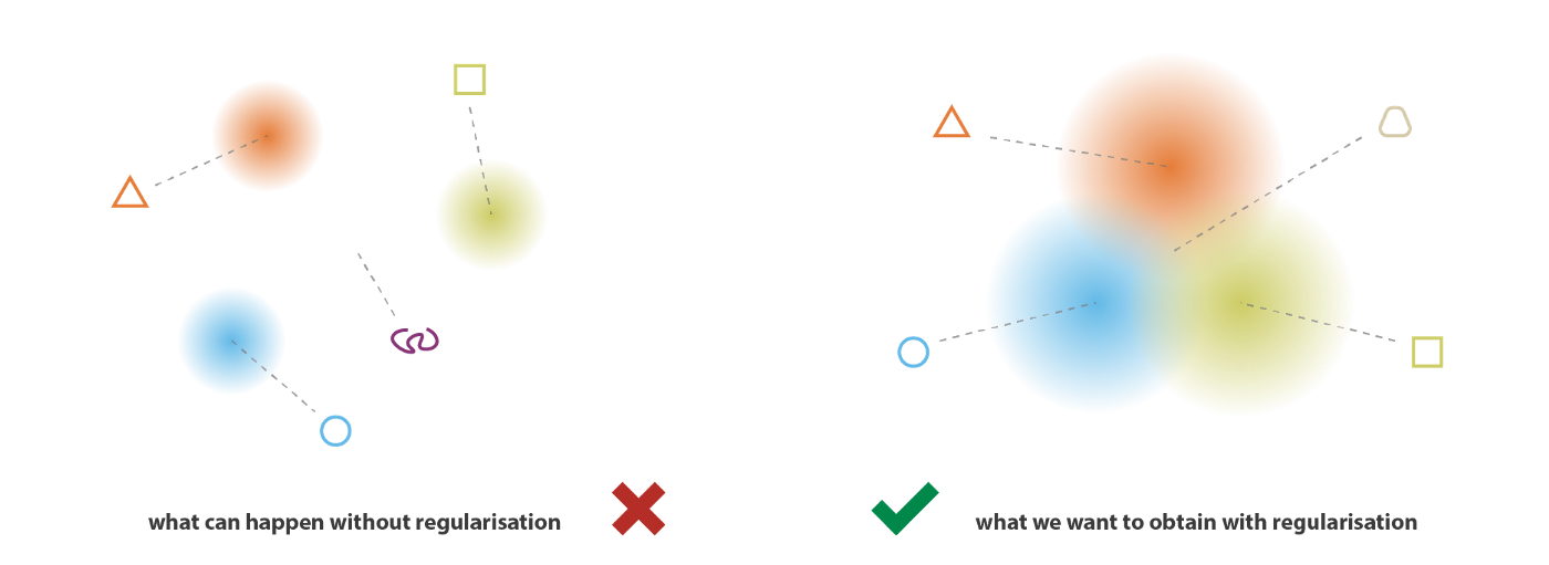
We construct normal code distributions using the encoded mean and variance. The assumption that $p(z|x)$ follows $\mathcal{N}(\mu,\sigma^2)$ can be seen as prior knowledge, but by itself it cannot prevent noise collapse. To make the generative process possible, we expect the latent space to have regularity. This regularity can be described through two main properties: continuity, meaning that two neighboring points in the latent space should not decode into completely different contents; and completeness, meaning that points sampled from the latent space under a given distribution should decode into “meaningful” contents.

Achieving continuity and completeness requires the code distributions of different samples $x$ to be as close as possible, while their variances should not be zero so that randomness in sampling is preserved, as shown in the following figure. By regularizing the code distributions, we can prevent the model’s codes in the latent space from drifting too far away from one another and encourage as many returned distributions as possible to overlap, thereby satisfying the expected continuity and completeness conditions.

On the other hand, the reconstruction error encourages the encoded content to preserve as much information as possible from the original sample, which leads to diversity in the code space. From this perspective, there is also a kind of adversarial idea in VAE, although it is relatively implicit and evolves jointly.

At a high level, this adversarial relationship can be described as follows. When the decoder is not sufficiently trained and the reconstruction loss is large, the network will reduce the noise, increasing the KL loss if we understand the typical case as $\sigma^2 <1$. The sampled $z$ becomes closer to the original data mean and contains more original information, which makes reconstruction easier. Conversely, when the decoder is well trained and the KL loss is large, the model needs to increase the noise, thereby reducing the KL loss. The variance becomes closer to 1, the sampling region becomes broader, and reconstruction becomes more difficult again. At that point, the decoder must further improve its reconstruction ability.

To summarize VAE: a VAE is an autoencoder that encodes input data as distributions rather than points, and its latent-space structure is regularized by constraining the distributions returned by the encoder to be close to the standard normal distribution.

Mathematical Origin of VAE

As mentioned above, VAE was introduced in the original paper in a somewhat supporting role, but its development since then is enough to show the effectiveness of its theory. Next, let us derive VAE from the perspective of the original paper.

The goal of the paper is to solve efficient inference in directed probabilistic graphical models. In large datasets, probabilistic graphical models often contain posterior distributions that are difficult to solve because of the large number of parameters. Similarly, for the autoencoding problem, given an observed dataset $X$, we want to infer the posterior distribution $p(z|x)$ of the code $z$ under the condition of a given sample $x\in X$.

As prior knowledge, we assume that the code distribution $p(z)$ belongs to a normal distribution. Then $p(z|x)$ is the encoder. To solve it, we can consider Bayes’ rule:

$$ p(z|x)=\frac{p(x|z)p(z)}{p(x)} $$

However, in Bayes’ rule, we cannot directly compute the denominator $p(x)$ and the likelihood $p(x|z)$, because according to the law of total probability, $p(x)=\int p(x|u)p(u)du$, and we cannot enumerate all possible $u$. In this situation, there are two possible ways to estimate $p(z|x)$:

Monte Carlo sampling, which we will not discuss here.
Variational inference.

The principle of variational inference is easy to understand. Since the original distribution $p(z|x)$ cannot be computed, we construct a new tractable distribution $q(z|x)$ to approximate it, making the two distributions as close as possible. KL divergence is used to measure the distance between these distributions.

Now, we use the distribution $q(z|x)$ to approximate the original distribution $p(z|x)$. Note that here $x$ refers to a specific sample selected from the dataset. The target we fit is the distribution dedicated to that sample. As prior knowledge, we assume that the code of the sample follows a normal distribution, $q(z|x)=\mathcal{N}(\mu_x,\sigma^2_x)$. Therefore, our objective becomes fitting the two parameters $\mu_x,\sigma^2_x$ of the code distribution given the sample $x$.

How do we fit them? With neural networks. We use $f(x)$ and $g(x)$ to fit $\mu$ and $\sigma^2$, respectively, or $\log \sigma^2$ as mentioned above. Thus, $q(z|x)=\mathcal{N}(f(x),g(x))$.

We want $q(z\mid x)$ to be as close as possible to $p(z\mid x)$, which means minimizing the KL divergence between the two distributions. In other words, we hope to find the optimal $f^*$ and $g^*$ such that

$$ \begin{aligned} (f^*,g^*) &= \operatorname*{arg\,min}_{f,g} \operatorname{KL}\left(q(z\mid x)\,\|\,p(z\mid x)\right) \end{aligned} $$

Before the derivation, let us recall what we are doing. We want to obtain the code distribution $p(z|x)$, but it cannot be computed directly, so we use $q(z|x)$ to approximate it. Up to this point, we have not really introduced VAE yet. Now let us begin the derivation:

$$ \begin{aligned} \operatorname{KL}\left(q(z\mid x)\,\|\,p(z\mid x)\right) &= \int q(z\mid x)\log \frac{q(z\mid x)}{p(z\mid x)}\,\mathrm{d}z \\ &= \int q(z\mid x)\log \frac{q(z\mid x)}{\frac{p(x\mid z)p(z)}{p(x)}}\,\mathrm{d}z \\ &= \int q(z\mid x)\log \left(q(z\mid x)\frac{p(x)}{p(x\mid z)p(z)}\right)\,\mathrm{d}z \end{aligned} $$

Expanding the expression according to the logarithm rule:

$$ \begin{aligned} \operatorname{KL}\left(q(z\mid x)\,\|\,p(z\mid x)\right) &= \int q(z\mid x)\log q(z\mid x)\,\mathrm{d}z {}+ \int q(z\mid x)\log p(x)\,\mathrm{d}z \\ &\quad - \int q(z\mid x)\log p(x\mid z)\,\mathrm{d}z {}- \int q(z\mid x)\log p(z)\,\mathrm{d}z \\ &= \log p(x) {}+ \int q(z\mid x)\log \frac{q(z\mid x)}{p(z)}\,\mathrm{d}z {}- \int q(z\mid x)\log p(x\mid z)\,\mathrm{d}z \end{aligned} $$

Now comes the key step:

$$ \begin{aligned} \operatorname{KL}\left(q(z\mid x)\,\|\,p(z\mid x)\right) &= \int q(z\mid x)\log \frac{q(z\mid x)}{p(z)}\,\mathrm{d}z {}- \int q(z\mid x)\log p(x\mid z)\,\mathrm{d}z {}+ \log p(x) \\ &= \operatorname{KL}\left(q(z\mid x)\,\|\,p(z)\right) {}- \mathbb{E}_{z\sim q(z\mid x)}\left[\log p(x\mid z)\right] {}+ \log p(x) \end{aligned} $$

This formula is powerful, so let us analyze it carefully. Overall, we hope to minimize the whole expression. That means the first KL-divergence term should be as small as possible, while the second expectation term should be as large as possible. As for the third term, although we do not know $p(x)$, once all samples are given, it is a constant and can be ignored during optimization.

Let us continue. The first KL-divergence term represents the distance between the assumed posterior distribution $q(z|x)$ and the prior distribution $p(z)$. In the original paper, $p(z)$ is assumed to be the standard normal distribution. The intuition is that a sufficiently expressive transformation can map normally distributed variables into very complex target distributions.

The second expectation term essentially says the following: for the distribution $q(z|x)$ that we use for approximation, given the code distribution generated from sample $x$, we sample $z$ from it, and the reconstruction $\hat{x}$ obtained using this $z$ should be as consistent as possible with the original sample. It may be easier to understand if we write it as:

$$ \mathbb{E}_{z\sim q(z\mid x)} \left[\log p(\hat{x}\mid z)\right] $$

The formula above tells us that, to make the assumed distribution $q(z|x)$ as consistent as possible with the posterior distribution $p(z|x)$, we need $q(z|x)$ to be close to the prior distribution $p(z)$. More importantly, we also need to reconstruct from the sampled $z$ so that the reconstructed result $\hat{x}$ is very likely to match the sample $x$. Since reconstruction is involved, we need to introduce a neural network, or some other model. In this way, we return to the architecture of an autoencoder.

Therefore, in short, the original motivation of VAE is to encode data with a distribution. But this distribution cannot be solved directly, so variational inference is required, and neural networks are used to fit an approximate distribution. This is also the meaning of the “V”, or Variational, in VAE. During the optimization of this approximating distribution, we need to optimize the fitting function through the reconstruction process of samples drawn from the code distribution. Therefore, a decoder is introduced, and the general AE architecture is formed.

Let us revisit the VAE loss function:

Continuing the analysis, the expectation term in the objective represents the distance between the generated result and the sample, which we measure using $||x-\hat{x}||^2$. The optimization term $KL(q(z|x)||p(z))$ has a concrete analytic form because the prior $p(z)$ is assumed to be a standard normal distribution. Meanwhile, we also assume $q(z|x)$ to be a normal distribution, whose parameters, namely variance and mean, are approximated by two neural networks: $\mu_x=f(x)$ and $\sigma_x^2=g(x)$. Therefore, we can also write the analytic expression involving $f$ and $g$. The KL term can be optimized as:

$$ \operatorname{KL}\left(\mathcal{N}(\mu,\sigma^2)\,\|\,\mathcal{N}(0,1)\right) = \frac{1}{2}\left(-\log \sigma^2 + \mu^2+\sigma^2-1\right) $$

Finally, we obtain the optimization function used in VAE:

$$ \operatorname{Loss} = \left\|x-\hat{x}\right\|^2 {}+\frac{1}{2}\left(-\log \sigma^2 + \mu^2+\sigma^2-1\right) $$